Scaling Time Series Forecasting with Facebook Prophet and SAS Viya
December 01, 2020
Time Series forecasting is one of the most challenging domains in Data Science and Machine Learning. To be successful, it requires a deep knowledge of the business, the data, the statistical methods as well as the right tools. In real-life use cases, to achieve reasonable levels of accuracy, we often need to build multiple models for hundreds of products at different levels of granularity, this leads to high levels of complexity and extensive processing times when using traditional tools.
We will see in this post how the deep domain expertise of SAS in Forecasting combined with the computation power of SAS Viya can help businesses overcome these challenges. To illustrate this we will use data from the M5 Competition on Kaggle.
The steps of this blog post were implemented on SAS Viya 3.5
Time Series Forecasting with Facebook Prophet
Prophet is an open source forecasting tool released by Facebook, it allows to model time series quickly and easily. It uses Stan under the hood for high-performance statistical computations and it is accessible in Python and R.

To use Facebook Prophet we start by dividing the data into separate time series, then the forecasting part is straightforward, here is a simple example of the modeling step, part of the code is from Matias’ blog post (see References). The full code is hosted on github.
from fbprophet import Prophet

def run_prophet(timeserie):
    model = Prophet()
    model.fit(timeserie)
    forecast = model.make_future_dataframe(periods=7)
    forecast = model.predict(forecast)
    return forecast
When we run this code locally on the local machine , it takes 13 hours and 30 minutes to run on 3049 time series.
Distributed processing on SAS Viya
SAS Viya allows to take the python code as is, and distribute it on its In-memory distributed engine CAS. In addition, it has a special method that takes the raw table as input as well as time series specific parameters and performs the separation/aggregation steps for us.

First, let’s see how we can run our code in a distributed way, then we will explain how it works in the next section.
To do so we write our python script with prophet modeling, it is similar to the previous code. We will call it python_prophet_code.py
from fbprophet import Prophet
import pandas as pd

# init DataFrame
df = pd.DataFrame({'ds': DS, 'y': Y})
df.ds = pd.to_timedelta(df.ds, unit='D') + pd.Timestamp('1960-1-1')

# Prophet Fit/Predict
m = Prophet()
m.fit(df.iloc[:(int(NFOR) - int(HORIZON))])
future = m.make_future_dataframe(periods=int(HORIZON))
forecast = m.predict(future)

# Output
PRED = np.array(forecast['yhat'])
Then, we define the variable cmpcode, it will encapsulate the definitions of inputs/outputs and logging variables, the most interesting part is the rc7 line that refers to our python script with the prophet code.
cmpcode = """
    declare object py(PYTHON3) ;
    rc1 = py.Initialize() ;

    rc2 = py.addVariable(Quantity, 'ALIAS', 'Y') ;
    rc3 = py.addVariable(date, 'ALIAS', 'DS') ;
    rc4 = py.AddVariable(PRED, "READONLY", "FALSE") ;
    rc5 = py.AddVariable(_LENGTH_, 'ALIAS', 'NFOR') ;
    rc6 = py.AddVariable(_LEAD_,'ALIAS','HORIZON') ;

    rc7 = py.PushCodeFile('
        /home/sahbic/python_prophet_code.py
        ');

    rc14 = py.Run() ;
    pyExitCode = py.GetExitCode() ;
    pyRuntime = py.GetRunTime() ;

    declare object pylog(OUTEXTLOG) ;
    rc15 = pylog.Collect(py, 'EXECUTION') ;
    declare object pyvars(OUTEXTVARSTATUS) ;
    rc16 = pyvars.collect(py) ;
 """
Finally, the function that does all the magic is the CAS action runTimeCode from the Time Series Processing Action Set (SAS users know it better under the name TSMODEL Procedure).
This method performs automatic forecast model generation, automatic variable and event selection, and automatic model selection.
Here we use it in a very special case to call the external python script.
# Load needed action sets
s.loadactionset(actionset="timedata")

# Time serires parameters
forecast_lead = 7
data_interval = "Day"
series_params = dict(accumulate='SUM', name='Quantity')

# helper function to make the action call code more clear
dname = lambda name: dict(name=name)

# Define and call the timedata.runTimecode action
res = s.timedata.runtimecode(
      table={'name':"M5_final",'caslib':'Public',
             'groupby':[dname("item_id")]},
      series=[series_params],
      interval=data_interval,
      require=dict(pkg="extlang"),
      timeid=dict(name='date'),
      lead=forecast_lead,
      arrayout={'arrays':[dname("PRED")],
                'table':dict(name="outarray", replace=True)},
      objout=[dict(table=dname("outobj_pylog"), objRef="pylog"),
              dict(table=dname("outobj_pyvars"), objRef="pyvars")],
      code=cmpcode)
When we run this code, it will run in a distributed way taking advantage of the available threads on the whole cluster.
In our configuration, with 32 threads, it takes 48 minutes and 55 seconds to run on the 3049 Time series. So we have a huge acceleration (16.5 speedup) !
How does it work ?
The action used in the previous section uses a special package called EXTLANG which enables integration with open source languages.
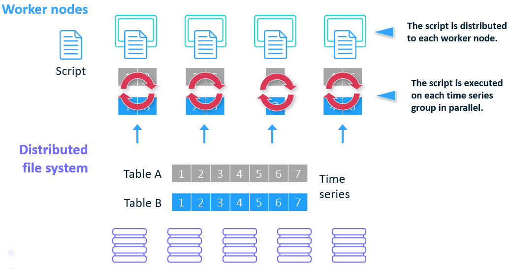
- The EXTLANG package allows to:
- Read multiple input data sets in parallel
- Distribute the execution of the open source code: each time series is executed on one thread of the computing node
- Logging if a problem occurs
- Have an efficient memory management strategy that minimizes the number of queries that are performed by the BY-group threads during the parallel execution step
- Write multiple output data sets in parallel
Conclusion
By leveraging the power of SAS Visual Forecasting on Viya, we reduce the processing time by a 16.5 ratio in our configuration.
SAS Viya enables us to create custom time series algorithms and processing steps to prepare the data for analysis, this all can be done in one single script and can be processed in a distributed way on a cloud infrastructure. This allows to accelerate the modeling and enable the data scientists and the business experts to leverage the data as well as the infrastructure at their disposal to create better forecasting models.
The full code is accessible on github.
References
- Scalable Cloud-Based Time Series Analysis and Forecasting Thiago Quirino, Michael Leonard, and Ed Blair, SAS Institute Inc
- Accelerate open source forecasting with SAS
- Forecasting multiple time-series using Prophet in parallel